What are GWAS Analysis Tools
This article provides an overview of key tools and methodologies used in GWAS, including an introduction to commonly used software, such as TASSEL, PLINK, and GEMMA, among others. It also guides researchers through the process of performing GWAS analysis, from data preparation to result visualization, using tools like QQ plots and Manhattan plots to interpret findings. Whether you are new to GWAS or an experienced researcher, this guide will provide valuable insights into the practical applications and best practices for conducting GWAS.
Introduction to GWAS
Genome-Wide Association Study (GWAS) is a research method used to analyze the associations between genotypes and phenotypes, widely applied in uncovering the genetic basis of complex traits. GWAS identifies genetic markers associated with specific diseases, traits, or other phenotypes, playing a significant role in disease prevention, drug development, and personalized medicine.
By analyzing genomic data from large sample populations, GWAS aims to pinpoint single nucleotide polymorphisms (SNPs) linked to particular traits. These associations may reveal potential biomarkers or guide future research directions.
Service you may intersted in
Key GWAS Analysis Tools
We have summarized information on commonly used GWAS analysis tools, including EMMAX, GEMMA, FarmCPU, PLINK, BLINK, MLM, SUPER, CMLM, MLMM, fastGWA, GenABEL, and FastLMM, in a table detailing their key features, computational speed, and publication year. Each software tool offers unique analytical advantages and is suited for specific scenarios. Selecting the most appropriate tool based on the specific research needs and data characteristics is crucial to ensuring the accuracy and reliability of GWAS analysis results.
| Software Name |
Key Features |
Computation Speed |
Publication Year |
Reference Link |
| EMMAX |
Based on the Mixed Linear Model (MLM), it accounts for population structure and kinship.
Supports rare variant analysis and genome-wide scans. |
Fast, optimized for large-scale data. |
2010 |
EMMAX Reference |
| GEMMA |
Supports both MLM and Generalized Linear Models (GLM).Adjusts for population structure and environmental effects.Handles binary and multi-class traits. |
Fast, efficient for large datasets. |
2012 |
GEMMA Reference |
| FarmCPU |
Combines MLM and Fixed Effect Models (FIXED). Improves detection accuracy for causal loci, especially in crop research. Improves detection accuracy for causal loci, especially in crop research. |
Moderate, optimized sparse matrix. |
2016 |
FarmCPU Reference |
| PLINK |
Designed for largescale genotype data quality control and GWAS analysis.Offers various statistical methods, including singlepoint associations and multiple corrections. |
Fast, particularly suited for preprocessing. |
2007 |
PLINK Reference |
| BLINK |
A GWAS tool optimized using Bayesian Information Criterion (BIC). Effectively detects signals with reduced false positive rates. |
Relatively fast, suitable for medium-scale data. |
2018 |
BLINK Reference |
| MLM(GAPIT3) |
Mixed Linear Model that accounts for population structure by incorporating random effects. |
Moderate, performance decreases with larger datasets. |
2021 |
GAPIT3 Reference |
| SUPER |
An optimized MLM approach using "Super Individuals" for modeling. Improves computational efficiency and reduces false positive rates. |
Fast, suitable for large-scale data. |
2014 |
SUPER Reference |
| CMLM |
Conditional Mixed Linear Model, an improvement over standard MLM. Enhances efficiency and accuracy in association detection. |
Moderate, slower as the number of conditions increases. |
2010 |
CMLM Reference |
| MLMM |
MultiLocus Mixed Model that incrementally adds fixed effects to improve GWAS signal detection. |
Moderate, suitable for small-to-medium datasets. |
2012 |
MLMM Reference |
| fastGWA |
Optimized implementation of MLM, designed for largescale human genomic studies. Capable of processing millions of samples and SNPs rapidly. |
Extremely fast, handles ultra-large datasets efficiently. |
2020 |
fastGWA Reference |
| GenABEL |
Rbased GWAS package. Provides a comprehensive solution from data quality control to association analysis. |
Slow, suitable for small datasets or exploratory studies. |
2007 |
GenABEL Reference |
| FastLMM |
A fast algorithm based on linear mixed models, optimized for sparse matrices. Supports singletrait and multitrait joint analysis. |
Fast, suitable for large-scale genotype data. |
2012 |
FastLMM Reference |
| TASSEL |
Integrates GLM and MLM for analysis, widely used in plant genetics research. Supports integrated analysis of phenotype, genotype, and environmental data. Provides both GUI and commandline modes. |
Fast, suitable for datasets of various sizes. |
2007 |
TASSEL Reference |
GWAS analysis by Tassel
Most of the aforementioned software requires a certain level of programming proficiency. However, TASSEL provides a complete compiled environment and installation package with a graphical user interface. As one of the earliest GWAS tools released, it is widely used in the field of plant genetics.
TASSEL offers comprehensive data processing, analysis, and visualization capabilities. The following outlines the detailed steps for conducting GWAS analysis using TASSEL.
1. Installation software
Installing TASSEL
Users need to first download the TASSEL 5 installation package from the official website or other reliable sources. There is a reliable website https://tassel.bitbucket.io.
This software can be installed under different operating systems, note that Mac OS needs to be installed under administrator rights, otherwise an error will be reported.
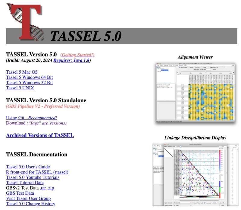 Fig. 1. TASSEL software download page.
Understanding software interface
File:Used to open and save data, as well as exit operations
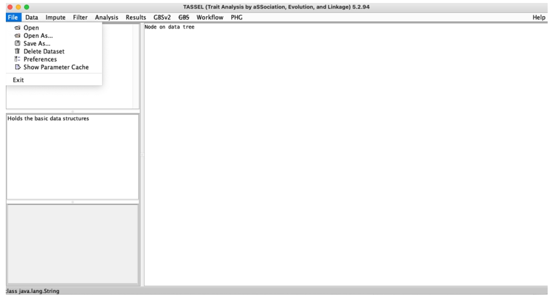 Fig. 2. TASSEL File menu.
Data:Perform operations on the imported data, such as sorting, intersection and union
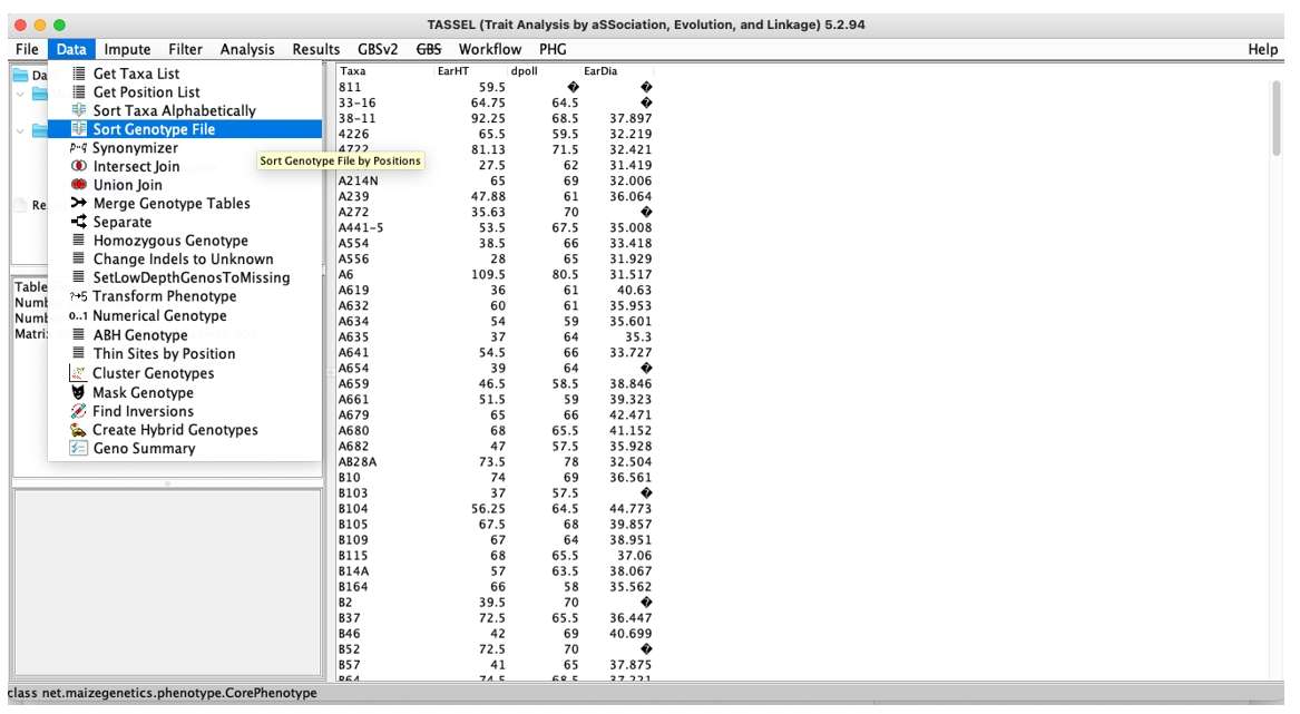 Fig. 3. TASSEL Data menu.
Impute:Fill data, including different fill methods.
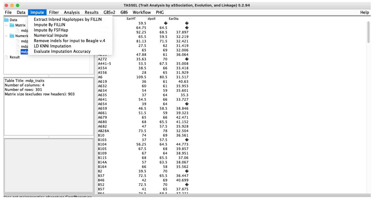 Fig. 4. TASSEL Impute menu.
Filter:Conduct data quality control.
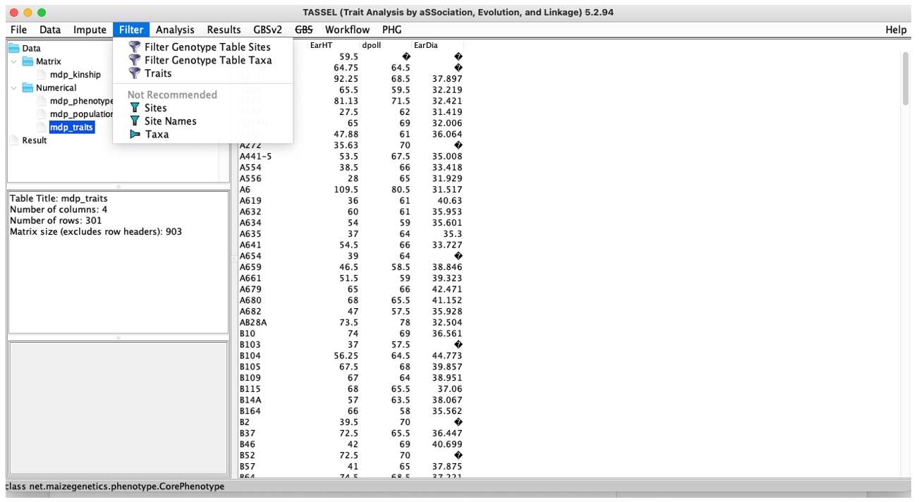 Fig. 5. TASSEL Filter menu.
Analysis:Are very major modules, including Kinship, PCA, MDS, Geno Summary methods, but also GLM (general linear model) and MLM (mixed linear model).
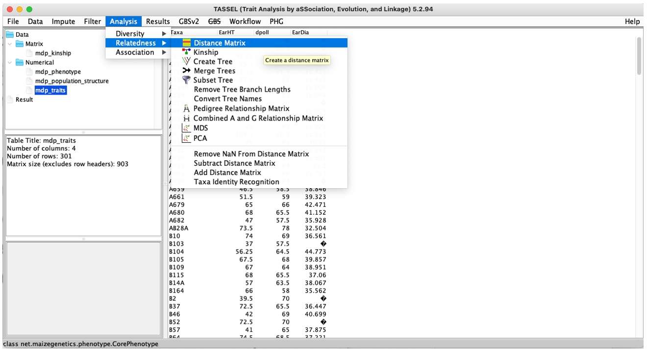 Fig. 6. TASSEL Analysis menu.
Results: Mainly is the result of visualization, including LD diagram, QQ diagram, Manhattan diagram and so on.
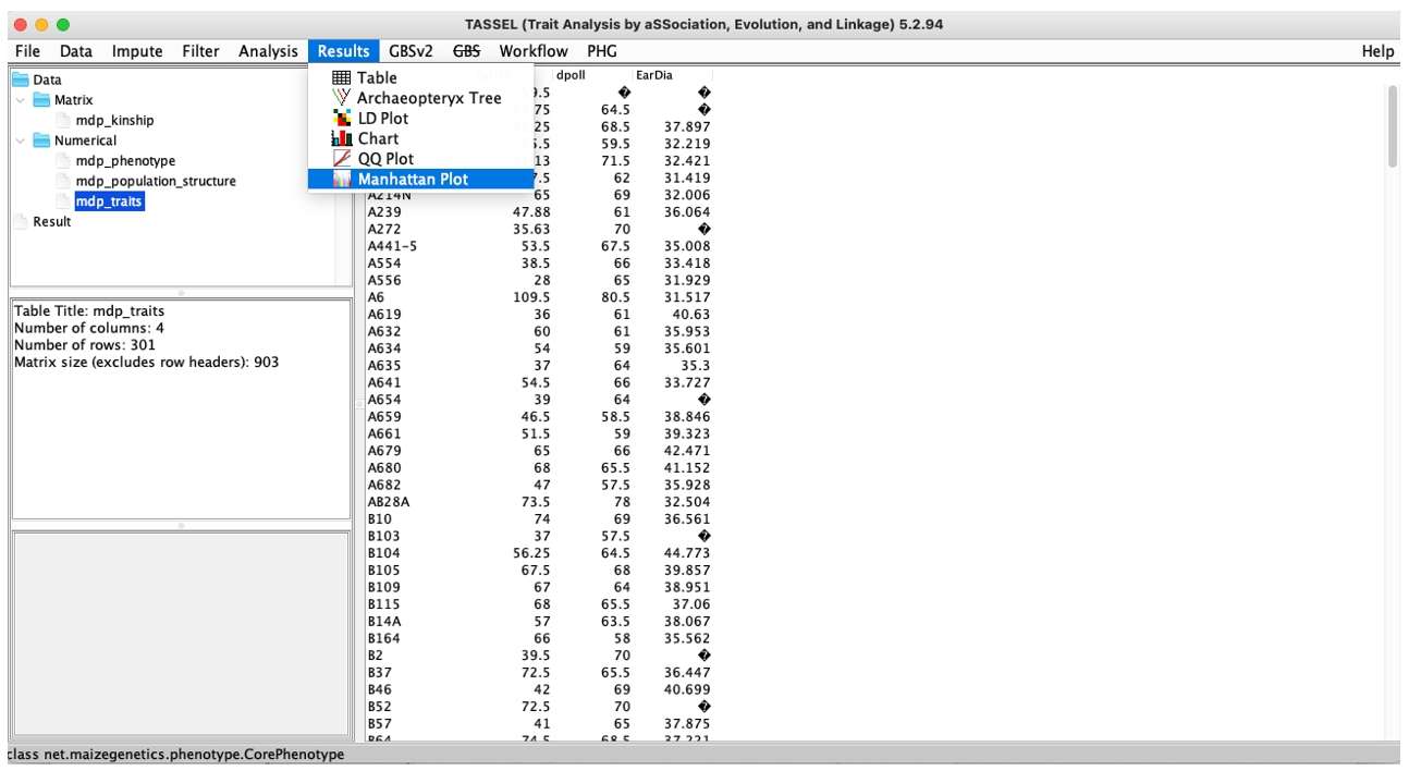 Fig. 7. TASSEL Results menu.
2.Data Import
Data Preparation
Four types of files are required for GWAS analysis
- Genotype File: Contains the genotype information of the samples, typically in Hapmap format.
- Kinship File: Used to analyze the kinship relationships between samples.
- Population Structure File: Used to assess the population structure of the samples.
- Phenotype File: Contains phenotype information corresponding to the samples, such as disease status or trait measurements.
The installation package of this software comes with a TutorialData folder, which contains the 4 necessary files for GWAS, and the file format is.txt.
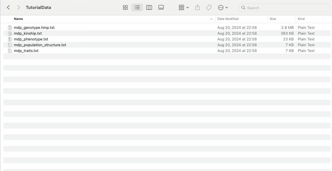 Fig. 8. TASSEL software TutorialDate foloder.
After opening the TASSEL software, the first step is to import the four types of data. Click on "File" in the toolbar and select "Open," which will provide options for importing data. Select the appropriate .txt file from a specific folder and then click "OK" to import the data.
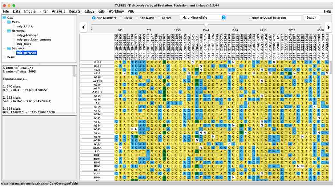 Fig. 9. TASSEL import genotype data.
When analyzing your own data, phenotype data is typically provided by the user, so attention should be paid to the format of the phenotype data. The first column in the file should contain the <Trait> label, the second column should include the traits to be analyzed, and the third column, along with subsequent columns, should represent the traits to be analyzed (one for each). The content under the <Trait> label should list the names of the materials being analyzed.
3.Data Quality Control
Genotype Data Quality Control:
Select the genotype data, then go to the "Filter" toolbar and click on "Sites." In the dialog box, click "Remove minor SNP states" and then click "Filter." This will generate the quality-controlled data, which will be used for subsequent analysis.
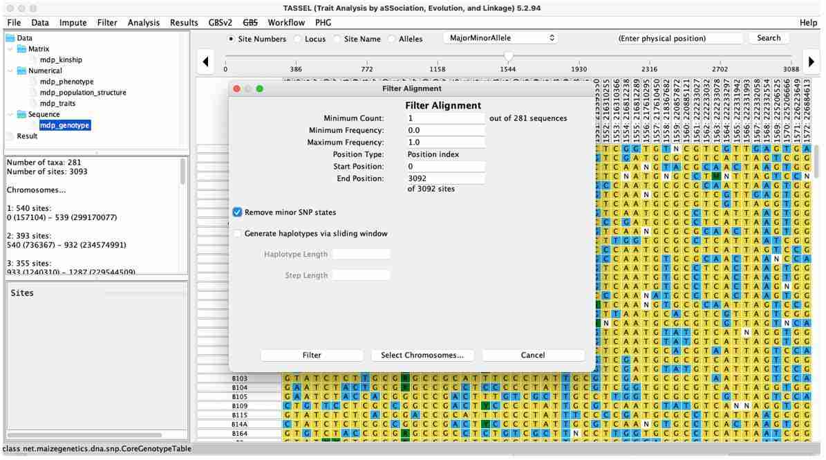 Fig. 10. TASSEL fliter genotype data.
Population Structure Data Quality Control:
Select the population structure data, then go to the "Filter" toolbar and click on "Traits." In the dialog box, change the "Type" column under "data" to "covariate," remove one checkmark under the "Include" column, and then click "OK." This will generate the quality-controlled population structure data.
4.GLM analysis
The Generalized Linear Model (GLM) is used for analyzing the Q model. When performing Q model analysis, three types of data are required: quality-controlled genotype data, quality-controlled population structure data, and phenotype data. Select these three datasets by holding down the Ctrl key, then go to the "Data" toolbar and click "Intersect Join." This will generate a new file, which contains the intersected data from the three datasets.
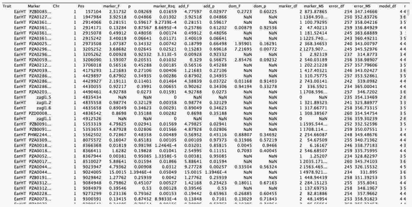
Select the intersected data, then go to the "Analysis" toolbar and click "GLM." In the dialog box that appears, click "OK" to generate the Q model result data, as shown in the table below.
5. Results visualization
To generate the QQ plot for the Q model, select the Q model result data, then go to the "Results" toolbar and click "QQ Plot." This will open a dialog box, where the left column contains the traits to be analyzed, and the right column shows the traits to be selected for analysis. Select a single trait to generate a single QQ plot, or select multiple traits to generate a combined QQ plot. Typically, a single trait is chosen. Then, click "Okay" to obtain the corresponding QQ plot. The plot can be saved by clicking the "save" button in the lower-right corner.
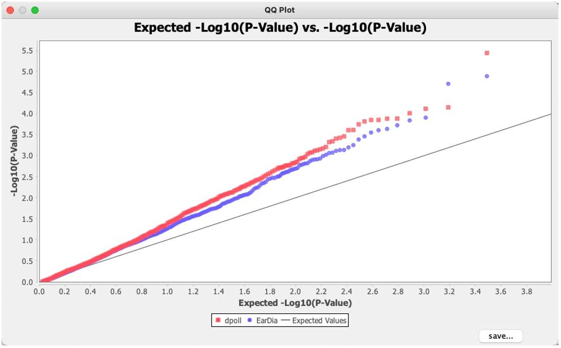 Fig. 11.QQ plot.
To generate the Manhattan plot for the Q model, select the Q model result data, then go to the "Results" toolbar and click "Manhattan Plot." This will open a dialog box. Click "Select trait" to choose a trait, then click "Okay" to generate the corresponding Manhattan plot. The plot can be saved by clicking the "save" button in the lower-right corner.
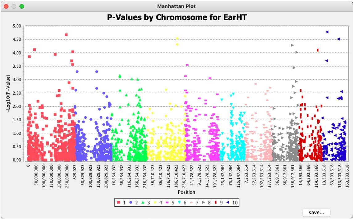 Fig. 12.Manhattan plot.
This is all about TASSEL, there are other model analysis, please feel free to explore more!
Reference:
-
Peter J. Bradbury, et.al. TASSEL: software for association mapping of complex traits in diverse samples, Bioinformatics, Volume 23, Issue 19, October 2007, Pages 2633–2635, https://doi.org/10.1093/bioinformatics/btm308

 Sample Submission Guidelines


